Policy gradient, PPO and GRPO
The RL Objective in the World of Large Language Models
The RL objective in the general RL world and in the world of large language models is essentially the same, though the expression is slightly different. Understanding this makes it easier to read articles from different RL settings. In particular:
- Articles from the general reinforcement learning world:
policy gradient,PPO - Articles from the large language model world:
DeepSeek R1,Kimi K1.5 technical report
In the general reinforcement learning setting, the algorithm optimizes the following objective:
\[ J(\pi_\theta) = \mathbb{E}_{\tau \sim \pi_\theta}[R(\tau)] = \mathbb{E}_{\tau \sim \pi_\theta}\left[\sum_{t=0}^{T} r_t\right] = \mathbb{E}_{\tau \sim \pi_\theta}\left[\sum_{t=0}^{T} r(s_t, a_t, s_{t+1})\right] \tag{1}\]
Here:
- \(\tau\) denotes a trajectory of
<state, action> - \(R(\tau)\) denotes the return, i.e. the cumulative reward, the sum of future rewards
- \(r_t = r(s_t, a_t, s_{t+1})\) denotes the reward function
However, in the world of large language models, the expression above can be updated and refined. The core reason is that the reward model does not provide a reliable and meaningful reward at every action step. We usually do not care about RM scores for intermediate results; we only care about the reward model’s score for the complete answer.
Therefore,
\[ r(s_t, a_t, s_{t+1}) = 0 \quad \text{for } t < T \tag{2}\]
\[ J(\pi_\theta) = \mathbb{E}_{\tau \sim \pi_\theta}\left[\sum_{t=0}^{T} r(s_t, a_t, s_{t+1})\right] = \mathbb{E}_{\tau \sim \pi_\theta}[r(s_T, a_T, s_{T+1})] \tag{3}\]
At the same time, if we let \(q\) denote the instruction (or question) seen by the model, and \(o\) denote the answer generated by the model, then \(o\) can be viewed as the trajectory \(\tau\) chosen by model \(\pi_\theta\):
\[ J(\pi_\theta) = \mathbb{E}_{q, o \sim \pi_\theta}[r(q, o)] \tag{4}\]
Here, \(r(q, o)\) denotes the score assigned by the reward model after seeing the user input and the model output.
The expectation in the expression above means: after optimization, for each question \(q\), the answer \(o\) produced by model \(\pi_\theta\) is likely to receive a higher reward from the reward model.
1. Policy Gradient
Policy gradient is an algorithm from the standard RL world. We first describe the problem and the solution using the language of general reinforcement learning, and define the objective function:
\[ J(\pi_\theta) = \mathbb{E}_{\tau \sim \pi_\theta}[R(\tau)] \tag{5}\]
The core derivation of its gradient is shown below:
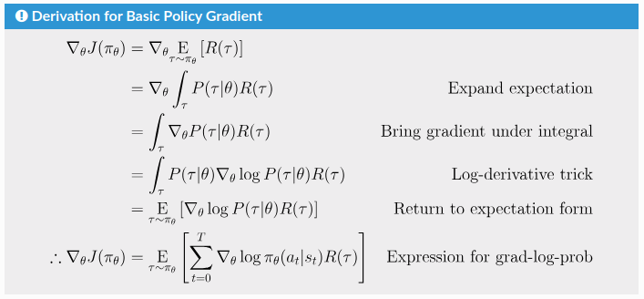
The gradient obtained above can be viewed as a weighted average of \(\nabla_\theta \log \pi_\theta\):
\[ \nabla_\theta \log \pi_\theta \cdot \text{weight} \tag{6}\]
Once we have the gradient, we basically arrive at a trainable and optimizable starting point. However, practice shows that training may be unstable, convergence may be slow, and performance may be suboptimal. Therefore, people introduced the concept of a baseline to improve stability and training efficiency.
In the policy gradient family of methods, the baseline is any term independent of the sampled action, used to reduce variance. It is used to subtract from the reward and adjust the weight on \(\nabla_\theta \log \pi_\theta\). After introducing the baseline, we obtain the core expression used in policy gradient methods:
\[ \nabla_\theta \log \pi_\theta \cdot (r - \text{baseline}) \tag{7}\]
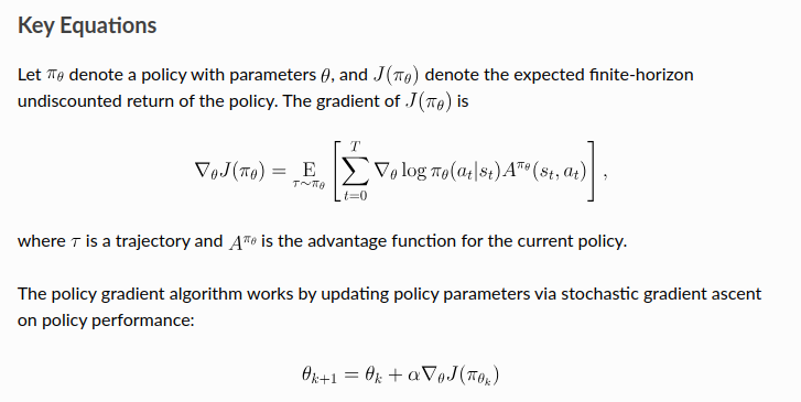
Under this formulation, the most common choice of weight is the advantage function, defined as:
\[ A^{\pi}(s, a) = Q^{\pi}(s, a) - V^{\pi}(s) \tag{8}\]
So the corresponding core gradient expression becomes:
\[ \nabla_\theta \log \pi_\theta \cdot A^{\pi} \tag{9}\]
Once we have this core gradient estimation form, vanilla policy gradient is essentially established:
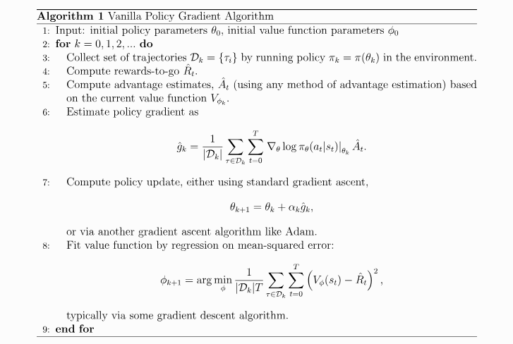
Up to this point, we have discussed the first column of the table below: policy gradient.
| Policy Gradient | PPO | GRPO | Kimi K1.5 | |
|---|---|---|---|---|
| policy model \(\pi_\theta\) | Required. This is the model being optimized. | Required. This is the model being optimized. | Required. This is the model being optimized. | Required. This is the model being optimized. |
| reference policy model \(\pi_{\theta_k}\) | Not required. | Required. | Required. | Required. |
| reward model | Required. | Required. | Required. | Required. |
| value function \(V_{\phi_k}\) (critic model) | Required. It estimates the expected future return, and methods such as GAE use it to compute the advantage. It must be continuously updated and kept accurate. | Required. It estimates the expected future return, and methods such as GAE use it to compute the advantage. It must be continuously updated and kept accurate. | Not required, because the computation of the advantage avoids this path. | Not required. Since the gradient can be written explicitly, the baseline-like term can be approximated by the sample mean. |
| rewards-to-go \(\hat{R}_t\) | Required, for updating the value function. | Required, for updating the value function. Exactly how the reward is distributed back to each token depends on the implementation. | Not needed, since there is no critic. | Not needed, since there is no critic. |
2. PPO
The PPO algorithm was proposed by Schulman (paper). It builds on ideas from policy gradient and trust region methods (TRPO).
As shown below, from the perspective of overall algorithmic structure, they are quite similar: both require a value function. The key difference lies in how the parameter \(\theta\) is updated. PPO introduces a new objective function, which leads to improvements in stability, convergence speed, performance, and ease of implementation.
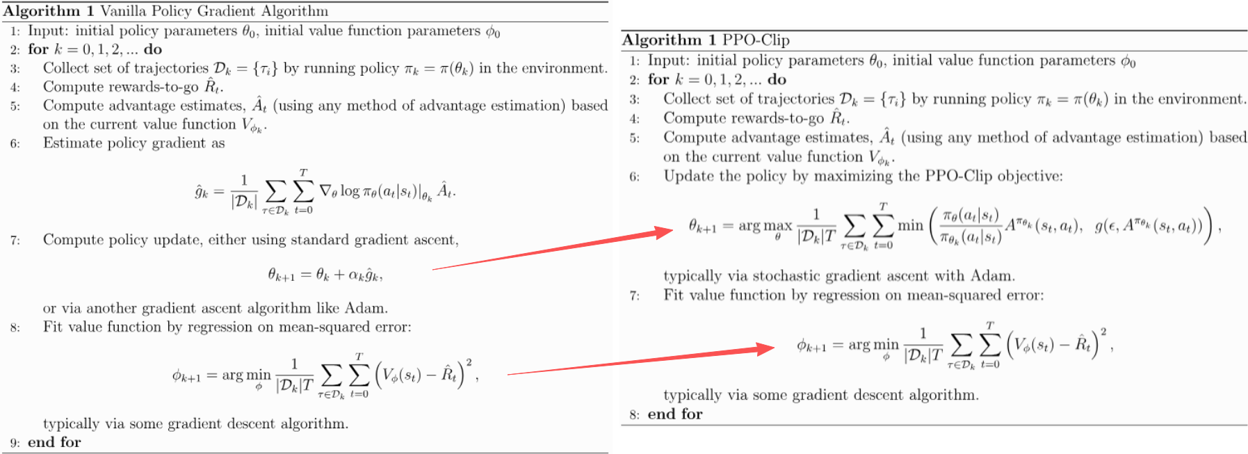
Unlike policy gradient, PPO does not directly solve the problem starting from the original objective:
\[ J(\pi_\theta) = \mathbb{E}_{\tau \sim \pi_\theta}[R(\tau)] \tag{10}\]
Instead, PPO uses a new objective, usually called the surrogate objective function. Its core term is:
\[ L_{\text{core}}(\theta) = \mathbb{E}_t \left[ \frac{\pi_\theta(a_t \mid s_t)}{\pi_{\theta_{\text{old}}}(a_t \mid s_t)} A_t \right] \tag{11}\]
The intuition is simple:
- If action \(a_t\) has positive advantage, then the new policy \(\pi_\theta\) should assign a higher probability to this action in the future.
- If action \(a_t\) has negative advantage, then the new policy should assign a lower probability to this action in the future.
GAE is a common method for estimating the advantage.
PPO’s objective does not stop here. It also adds a clipping term:
\[ \operatorname{clip}\left( \frac{\pi_\theta(a_t \mid s_t)}{\pi_{\theta_{\text{old}}}(a_t \mid s_t)}, 1 - \epsilon,\ 1 + \epsilon \right) A_t \tag{12}\]
The idea is to prevent the model from changing too much in a single update, so that training does not become overly aggressive.
Then the new objective includes one more step:
\[ \min\left( \frac{\pi_\theta(a_t \mid s_t)}{\pi_{\theta_{\text{old}}}(a_t \mid s_t)} A_t,\ \operatorname{clip}(\cdot) A_t \right) \tag{13}\]
This makes the optimization behaviour more complicated. Readers are encouraged to analyze the behavior when \(A_t\) is positive or negative, and when the ratio \(\frac{\pi_\theta(a_t \mid s_t)}{\pi_{\theta_{\text{old}}}(a_t \mid s_t)}\) is greater than \(1 + \epsilon\) or less than \(1 - \epsilon\).
The full PPO objective is therefore:
\[ L(\theta)=\mathbb{E}_t\left[ \min\left( \frac{\pi_\theta(a_t \mid s_t)}{\pi_{\theta_{\text{old}}}(a_t \mid s_t)} A_t,\ \operatorname{clip}\left( \frac{\pi_\theta(a_t \mid s_t)}{\pi_{\theta_{\text{old}}}(a_t \mid s_t)}, 1-\epsilon,\,1+\epsilon \right)A_t \right) \right] \tag{14}\]
This new objective does not have a closed-form solution, so it is optimized through stochastic gradient ascent.
So far, we have discussed the second column of the table below: PPO.
| Policy Gradient | PPO | GRPO | Kimi K1.5 | |
|---|---|---|---|---|
| policy model \(\pi_\theta\) | Required. This is the model being optimized. | Required. This is the model being optimized. | Required. This is the model being optimized. | Required. This is the model being optimized. |
| reference policy model \(\pi_{\theta_k}\) | Not required. | Required. | Required. | Required. |
| reward model | Required. | Required. | Required. | Required. |
| value function \(V_{\phi_k}\) (critic model) | Required. It estimates the expected future return, and methods such as GAE use it to compute the advantage. It must be continuously updated and kept accurate. | Required. It estimates the expected future return, and methods such as GAE use it to compute the advantage. It must be continuously updated and kept accurate. | Not required, because the computation of the advantage avoids this path. | Not required. Since the gradient can be written explicitly, the baseline-like term can be approximated by the sample mean. |
| rewards-to-go \(\hat{R}_t\) | Required, for updating the value function. | Required, for updating the value function. Exactly how the reward is distributed back to each token depends on the implementation. | Not needed, since there is no critic. | Not needed, since there is no critic. |
3. GRPO
GRPO is very similar to PPO. To better see the difference, we first need to understand one detail in the mathematical expression. The mathematics in the GRPO paper is written in the style of the LLM setting. The core idea is that it no longer focuses on the ratios or advantages associated with intermediate steps \(t < T\), and only cares about the final step \(t = T\). As a result, in the objective, the expectation over \(t\) in the form \(\mathbb{E}_t[\cdots]\) no longer appears.
Next comes the key extension in GRPO: it introduces repeated sampling for the same prompt \(q\). For a given prompt \(q\), the model performs multiple rollouts and obtains a group of outputs \(\{o_1, o_2, \ldots, o_G\}\). GRPO then uses this group of outputs to define the advantage and the optimization direction. This is the main innovation of GRPO.
More specifically, given a prompt \(q\), GRPO samples a group of outputs \(\{o_1, o_2, \ldots, o_G\}\) from the reference policy \(\pi_{\theta_{\text{old}}}\). The new policy is then optimized so that, within this group, outputs with above-average advantage are encouraged. Ignoring the KL term, the objective can be written as:
\[ L(\theta)=\mathbb{E}_{q}\left[ \min\left( \frac{\pi_\theta(o \mid q)}{\pi_{\theta_{\text{old}}}(o \mid q)}A_o,\ \operatorname{clip}\left( \frac{\pi_\theta(o \mid q)}{\pi_{\theta_{\text{old}}}(o \mid q)},\,1-\epsilon,\,1+\epsilon \right)A_o \right) \right] \tag{15}\]
The structure of this objective is the same as PPO. In practice, the expectation above is implemented as an average over the \(G\) sampled outputs:
\[ L(\theta)=\frac{1}{G}\sum_{i=1}^{G}\left[ \min\left( \frac{\pi_\theta(o_i \mid q)}{\pi_{\theta_{\text{old}}}(o_i \mid q)}\hat{A}_i,\ \operatorname{clip}\left( \frac{\pi_\theta(o_i \mid q)}{\pi_{\theta_{\text{old}}}(o_i \mid q)},\,1-\epsilon,\,1+\epsilon \right)\hat{A}_i \right) \right] \tag{16}\]
Unlike PPO, the advantage here is not estimated with GAE. Instead, it is computed by normalizing the rewards \(\{r_i(q_i, o)\}\) within the group:
\[ \hat{A}_i=\frac{r_i-\bar{r}}{\operatorname{std}(\{r_1,\ldots,r_G\})} \tag{17}\]
Under this design, there is no longer a need for a critic model or for GAE-based advantage estimation. This reduces computation cost and also avoids relying on a separately trained critic model whose estimates may be inaccurate, thereby reducing one source of instability.
So far, we have discussed the third column of the table below: GRPO.
| Policy Gradient | PPO | GRPO | Kimi K1.5 | |
|---|---|---|---|---|
| policy model \(\pi_\theta\) | Required. This is the model being optimized. | Required. This is the model being optimized. | Required. This is the model being optimized. | Required. This is the model being optimized. |
| reference policy model \(\pi_{\theta_k}\) | Not required. | Required. | Required. | Required. |
| reward model | Required. | Required. | Required. | Required. |
| value function \(V_{\phi_k}\) (critic model) | Required. It estimates the expected future return, and methods such as GAE use it to compute the advantage. It must be continuously updated and kept accurate. | Required. It estimates the expected future return, and methods such as GAE use it to compute the advantage. It must be continuously updated and kept accurate. | Not required, because the computation of the advantage avoids this path. | Not required. Since the gradient can be written explicitly, the baseline-like term can be approximated by the sample mean. |
| rewards-to-go \(\hat{R}_t\) | Required, for updating the value function. | Required, for updating the value function. Exactly how the reward is distributed back to each token depends on the implementation. | Not needed, since there is no critic. | Not needed, since there is no critic. |
Why a Critic Can Suppress Reflective CoT (long CoT)
DeepSeek-style methods and Kimi K1.5 both remove the critic, that is, the value function. Beyond computational efficiency, one important motivation is related to reflective CoT, or long chain-of-thought reasoning.
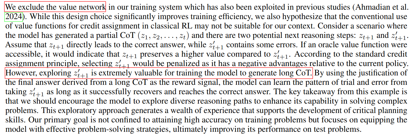
Recent reasoning-focused LLM work suggests that strong reasoning often involves exploring intermediate paths that may look locally unpromising, partially wrong, or unnecessarily long. Even so, these paths can still be useful if they eventually lead to a correct or insightful final answer.
A critic, however, is trained to estimate expected future return from intermediate states. In principle, this means it may assign low value to reasoning paths that do not look promising early on. If that happens, the policy may be discouraged from exploring those paths, even when they would have been useful in the full sequence.
From this perspective, removing the critic is not only a computational simplification. It also avoids relying on an intermediate value estimate that may prematurely suppress exploratory reasoning.
Main references:
- RL Basics: Spinning Up Part 1: Key Concepts in RL
- Policy Gradient Theory Basics: Spinning Up Part 3: Intro to Policy Optimization
- Basic Version of Policy Gradient: Spinning Up - Vanilla Policy Gradient
- PPO: Spinning Up - Proximal Policy Optimization
- Schulman’s PPO paper: PPO Algorithm
- GAE: High-Dimensional Continuous Control Using Generalized Advantage Estimation
- GRPO: